TensorFlow Logistic Regression
19 Sep 2017
What is the best way to start explaining what is logistic regression?
As you have learned about linear regression, its easier to compare and contrast it with logisitic regression to get satrted.
In linear regression, you have a set of parameters which define the problem and a cost function which needs to be optimized as per need.
Here once the model is trained , you mostly get continuous distribution of output (1, 1.5, 5, 1.3, 3.7., 97) in any range. Which means you can get any number as the prediction based on the constraints provided.
On the other hand, once you train a logistic regression model ; you only get a discrete set of binary values i.e 0 or 1. Once you satrt thinking about it, you will understand that logistic regression is able to answer only YES or NO questions. For example, you can’t go 1/2 to the party, you either go or you don’t. That’s logistical reasoning.
Why is it called logistic ‘regression’?
There is nothing as complicated in it, other than it’s name.
Logistic regression, despite its name, is a linear model for classification rather than regression. Logistic regression is also known in the literature as logit regression, maximum-entropy classification (MaxEnt) or the log-linear classifier. In this model, the probabilities describing the possible outcomes of a single trial are modeled using a logistic function.
Whenever you have a variable which is dependent on other variable(s), then you can map a mathematical relationship between them. When this relationship is lnear in nature, then you get linear equations(which leads to linear regression), whereas if you have a non- linear relationship which maps any input to a 0 or 1 then it is logistic in nature.
The process followed to determine this relationship between 2 or more variables where a change in a dependent variable is associated with a change in one or more independent variables, is regression.
To better understand logistic regression, its vital to know the logistic/sigmoid function.
Sigmoid Function
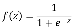
An explanation of logistic regression can begin with an explanation of the sigmoid function. The sigmoid function is useful because it can take any real input t, whereas the output always takes values between zero and one and hence is interpretable as a probability. The sigmoidfunction sigma(z) is defined as follows:
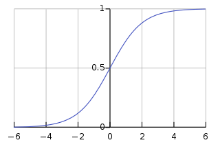
The Sigmoid(x) function goes to 0 as x goes to −∞ and to 1 as x goes to +∞
MNIST Example
1. Import Libraries
import tensorflow as tf

# Import MINST data
from tensorflow.examples.tutorials.mnist import input_data
mnist = input_data.read_data_sets("/tmp/data/", one_hot=True)
Extracting MNIST_data/train-images-idx3-ubyte.gz
Extracting MNIST_data/train-labels-idx1-ubyte.gz
Extracting MNIST_data/t10k-images-idx3-ubyte.gz
Extracting MNIST_data/t10k-labels-idx1-ubyte.gz
2. Set Learning parameters
# Parameters
learning_rate = 0.01
training_epochs = 25
batch_size = 100
display_step = 1
3. Create the Logistic Regression model graph
# tf Graph Input
x = tf.placeholder(tf.float32, [None, 784]) # mnist data image of shape 28*28=784
y = tf.placeholder(tf.float32, [None, 10]) # 0-9 digits recognition => 10 classes

# Set model weights
W = tf.Variable(tf.zeros([784, 10]))
b = tf.Variable(tf.zeros([10]))

# Construct model
pred = tf.nn.softmax(tf.matmul(x, W) + b) # Softmax

# Minimize error using cross entropy
cost = tf.reduce_mean(-tf.reduce_sum(y*tf.log(pred), reduction_indices=1))
# Gradient Descent
optimizer = tf.train.GradientDescentOptimizer(learning_rate).minimize(cost)

# Initialize the variables (i.e. assign their default value)
init = tf.global_variables_initializer()
4. Start training the model
# Start training
with tf.Session() as sess:
    sess.run(init)

    # Training cycle
    for epoch in range(training_epochs):
        avg_cost = 0.
        total_batch = int(mnist.train.num_examples/batch_size)
        # Loop over all batches
        for i in range(total_batch):
            batch_xs, batch_ys = mnist.train.next_batch(batch_size)
            # Fit training using batch data
            _, c = sess.run([optimizer, cost], feed_dict={x: batch_xs,
                                                          y: batch_ys})
            # Compute average loss
            avg_cost += c / total_batch
        # Display logs per epoch step
        if (epoch+1) % display_step == 0:
            print "Epoch:", '%04d' % (epoch+1), "cost=", "{:.9f}".format(avg_cost)

    print "Optimization Finished!"
5. Test the learned model graph
    # Test model
    correct_prediction = tf.equal(tf.argmax(pred, 1), tf.argmax(y, 1))
    # Calculate accuracy for 3000 examples
    accuracy = tf.reduce_mean(tf.cast(correct_prediction, tf.float32))
    print "Accuracy:", accuracy.eval({x: mnist.test.images[:3000], y: mnist.test.labels[:3000]})
Epoch: 0001 cost= 1.182138959
Epoch: 0002 cost= 0.664778162
Epoch: 0003 cost= 0.552686284
.
.
.
Epoch: 0014 cost= 0.367308579
Epoch: 0015 cost= 0.362704660
Epoch: 0016 cost= 0.358588599
Epoch: 0017 cost= 0.354823110