Machine Learning - II

15 Apr 2017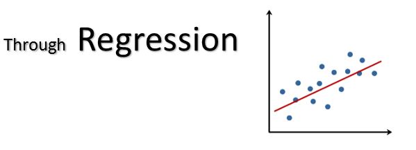

Now after considering the previous example of classification, let’s explore regression.

Assume you have some labelled training data consisting of various housing prices based on their square footage. Now if we plot our data we may get something like this:

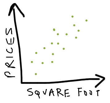
Each x’s represents a unique house with its corresponding price and square footage.

Even though our data is scattered over the space of the graph, still it follows some basic pattern: here the prices increase as the size does. So we want our learning algorithm to do this prediction for us i.e. we supply the square footage and the algorithm gives out prices.

The generally visible trend would be a diagonal passing through the mean (x, y) positions of the data. Every such line which give a sufficiently good fit to the data, is called a predictor.

You can call regression as a form of glorified curve fitting.

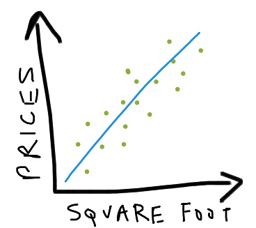
Once we get this predictor, we can guess with a bit more conviction that a house of size ‘a’ will have prices xxxx. Most houses in our training data are at the lowest possible distance from the predictor. This simply implies that all houses will have a high probability of lying on the diagonal learned.

We can have a number of linear trends to map our data:

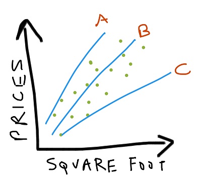
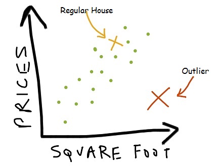
So any house which is not adhering to this predictor is either an outlier or doesn’t actually exist!

Now how we decide which is the best predictor, based on some quantized metric?

Error metric: absolute difference (L1 norm), squared difference (L2 norm)

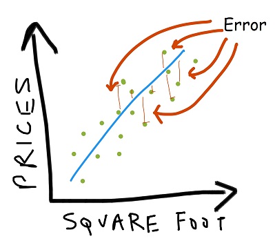
Once we get an error metric for each such possible predictor, we need to optimize it and then compare it with other alternatives.

For optimizing there are various techniques and algorithms possible to be implemented. More on that in another detailed post.

Also to add it’s not necessary for a predictor to be linear in nature. It can be of any degree. Quadratic, sinusoidal and even random unknown function work well.

Now if we look back at our housing price example, we just considered a single parameter – square footage. Why not extend our model by including more parameters like floor, parking space availability, amenities and age of house. Including most factors which influence the price of a house, will help us achieve higher accuracy of our predictor.

If you are not used to visualizing a multi-axis plot, then it appear a bit confusing at the start.

Just to spur your imagination, consider our simple square footage based estimator vs price. Here we had the prices along the y-axis and the square footage along the x-axis. Now as you keep increasing the dimensions (parameters) of your model, then subsequently more mutually orthogonal planes would start being added to our plot.

We consider a 2 parameter model, for which the graph will appear something like this:

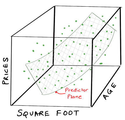
Again in this case we can have a predictor fit to our training data, but instead of a line, we need to draw a plane through the data because

plane = f(size, age) and equivalently our previous example was line = f(size)

Simply put, it has 2 input variables. There are a lot of other machine learning use cases which take into account hundreds or even around 1000s of variables. Sadly we can’t easily visualize any higher than 3 dimension, still can apply the above concepts to such systems.