Gradient Descent

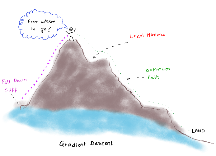
Hello guys,

Everyone is required to use some sort of algorithm to optimize the machine learning model parameters. What would be the best way to quickly get the optimum values of weights and bias such that the model converges quickly, but still doesn’t overfit the training data?

This post tries to explain one such optimization algorithm gradient descent through intuitive examples first, and then dives into the mathematics behind it. Hence feel free to jump to any section which interests you.

Intuition

Consider a situation, when you need to climb down a mountain but you don’t have an exact map of the way down. Anyways you need to get down so better start moving in some direction right?
So you start climbing down from the side where there is more slope, so that you reach the bottom quickly but safely.

Now there are two possible scenarios here:

1. You take very large steps, which ultimately leads you to a fall down a cliff
2. You take tiny steps, and this takes you so long to reach that you may or may not survive till then.

This obviously you don’t want and need. What to do then?

Simply walk like you do normally, but be attentive for down-direction.

Explanation

Until now we have just had a conceptual understanding of gradient descent algorithm, now let’s jump into the mathematics behind it.

Suppose you have a function which defines how close or far you are from achieving your learning goal. This function is called the cost function, here we represent it by J.

The role of gradient descent is to minimize this cost function J, so that we reach the most optimal solution. Though it isn’t necessary that we will always reach the global minima.

To ensure that we reach the best possible one, we need to make certain changes in our approach which we will discuss later in this post.

Gradient descent is used in machine learning for minimization of the cost.

In general let us consider a cost function like

J(θ1, θ2), and we want to find out min J(θ1, θ2).

Pseudo algorithm for Gradient Descent

1. Start with an initial guess

   • starting at 1,1; or 0,0 or any other value of choice
   • try and reduce J(θ1, θ2) by changing θ1 and θ2

2. Every change in parameter should be such that you select a gradient which reduces J(θ1, θ2) by the maximum possible difference

3. Repeat steps 1 and 2

4. Continue this until you converge to a local minimum

It’s really interesting to know that the point at which you start can lead you to a different minimum every time.

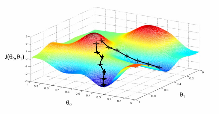
Here it’s visible that one initialization point led to once local minimum and the other led to a different one!

Some mathematics

All what we have understood above is equivalent to doing the following until convergence:

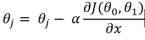
This simple means, we need to update θj by repeatedly updating it to θj - α times the partial derivative of the cost function with respect to θj.

Here, α is the learning rate which controls how big or small step you take in successive iteration.

1. If α is very small, then the tiny steps will lead to a long convergence time for the cost function

2. If α is very large, then you will aggressively reduce the value of θj

We need to select α such that the steps are neither too small nor too big so as to miss the optimal solution.

Variants

There are many variants of gradient descent used for machine learning.

Three of the highly used variants are as follow:

1. Batch Gradient Descent

The gradient descent algorithm by default is the batch gradient descent, which computes the gradient of the cost function wrt θj by taking into consideration the entire training dataset.

Since we are required to calculate gradient for the whole dataset for performing one update, it can be very slow and unmanageable for datasets which cant fit into memory.

Psuedocode for batch gradient descent:

for j in range(nb_epochs):
	grad_params = calculate_gradient(cost_function, training_data, params)
    	params = params - learning_rate * grad_params
  

Once the above process has been carried out, we update our parameters in the direction of the gradients. Batch gradient descent is guaranteed to converge to global minima for convex cost functions and to local minimas for non-convex costs.

2. Stochastic Gradient Descent (SGD)

In stochastic gradient descent performs an update for each training example. Batch gradient descent, in a way recomputes gradients for similar examples before each parameter update. And SGD eliminates this redundancy by performing one update at a time. So it is much faster to converge.

Psuedocode for stochastic gradient descent:

for j in range(nb_epochs):
	for example_i in data:
		grad_params = calculate_gradient(cost_function, example_i, params)
    		params = params - learning_rate * grad_params
  

Due to repeated updates to the parameters, the SGD cost function fluctuates alot which may lead to finding new better local minimas than the global minima granted by batch gradient descent. But this fluctuation also leads to difficulty in converging to exact mimima as SGD keeps overshooting. This can be removed by slowly reducing the learning rate as the number of updates increase.

3. Mini-batch Gradient Descent

Like in batch gradient descent we consider the entire training set before each update, similarly in mini-batch gradient descent we only take into consideration a limited number of examples for each update i.e. we update based on a min-batch of n training examples.

Psuedocode for mini-batch gradient descent:

for j in range(nb_epochs):
  np.random.shuffle(data)
  for batch in get_batches(data, batch_size=20):
  	grad_params = evaluate_gradient(loss_function, batch, params)
	params = params - learning_rate * grad_params
  

Such an implementation reduces the variance of parameters, which in turn can lead to more stable convergence. Mini-batch gradient descent is the choice of variant for neural networks, with a sizes ranges between 50 and 256. People are also used to the term SGD even when actually mini-batch gradient descent is being used.

Stay tuned for more machine learning and neural networks insight!